Unit 2.3
Data connections, trends, and correlation. Pandas is introduced as it could be valuable for PBL, data validation, as well as understanding College Board Topics.


- Files To Get
- Pandas and DataFrames
- Cleaning Data
- Extracting Info
- Create your own DataFrame
- Example of larger data set
- APIs are a Source for Writing Programs with Data
- Hacks
Files To Get
Save this file to your _notebooks folder
Save these files into a subfolder named files in your _notebooks folder
wget https://raw.githubusercontent.com/nighthawkcoders/APCSP/master/_notebooks/files/data.csv
wget https://raw.githubusercontent.com/nighthawkcoders/APCSP/master/_notebooks/files/grade.json
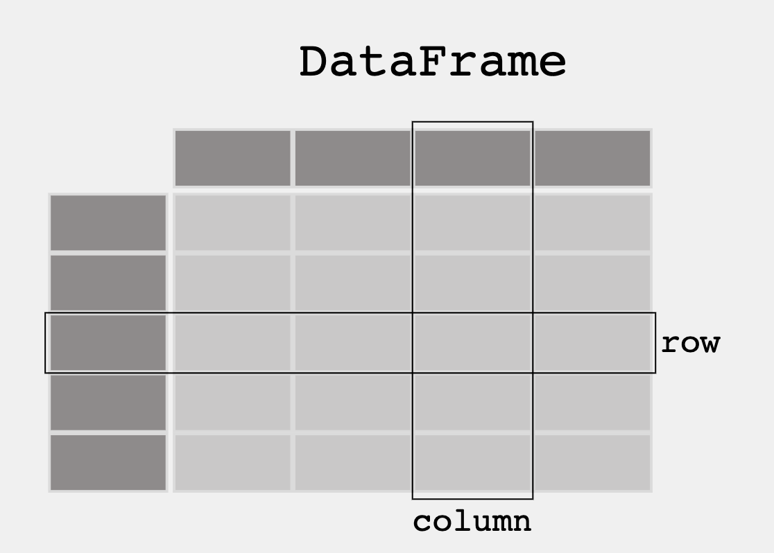
Save this image into a subfolder named images in your _notebooks folder
wget https://raw.githubusercontent.com/nighthawkcoders/APCSP/master/_notebooks/images/table_dataframe.png
Pandas and DataFrames
In this lesson we will be exploring data analysis using Pandas.
- College Board talks about ideas like
- Tools. "the ability to process data depends on users capabilities and their tools"
- Combining Data. "combine county data sets"
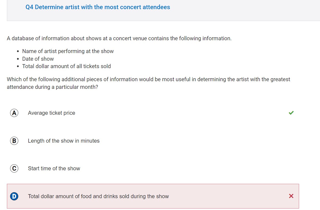
- Status on Data"determining the artist with the greatest attendance during a particular month"
- Data poses challenge. "the need to clean data", "incomplete data"
- From Pandas Overview -- When working with tabular data, such as data stored in spreadsheets or databases, pandas is the right tool for you. pandas will help you to explore, clean, and process your data. In pandas, a data table is called a DataFrame.
'''Pandas is used to gather data sets through its DataFrames implementation'''
import pandas as pd
df = pd.read_json('grade.json')

print(df)
# What part of the data set needs to be cleaned?
# From PBL learning, what is a good time to clean data?  Hint, remember Garbage in, Garbage out?
print(df[['GPA']])

print()

#try two columns and remove the index from print statement
print(df[['Student ID','GPA']].to_string(index=False))
print(df.sort_values(by=['GPA']))

print()

#sort the values in reverse order
print(df.sort_values(by=['GPA'], ascending=False))
print(df[df.GPA > 3.00])
print(df[df.GPA == df.GPA.max()])
print()
print(df[df.GPA == df.GPA.min()])
import pandas as pd

#the data can be stored as a python dictionary
dict = {
  "calories": [420, 380, 390],
  "duration": [50, 40, 45]
}
#stores the data in a data frame
print("-------------Dict_to_DF------------------")
df = pd.DataFrame(dict)
print(df)

print("----------Dict_to_DF_labels--------------")

#or with the index argument, you can label rows.
df = pd.DataFrame(dict, index = ["day1", "day2", "day3"])
print(df)
print("-------Examine Selected Rows---------")
#use a list for multiple labels:
print(df.loc[["day1", "day3"]])

#refer to the row index:
print("--------Examine Single Row-----------")
print(df.loc["day1"])
print(df.info())
import pandas as pd

#read csv and sort 'Duration' largest to smallest
df = pd.read_csv('files/data.csv').sort_values(by=['Duration'], ascending=False)

print("--Duration Top 10---------")
print(df.head(10))

print("--Duration Bottom 10------")
print(df.tail(10))
'''Pandas can be used to analyze data'''
import pandas as pd
import requests

def fetch():
    '''Obtain data from an endpoint'''
    url = "https://flask.nighthawkcodingsociety.com/api/covid/"
    fetch = requests.get(url)
    json = fetch.json()

    # filter data for requirement
    df = pd.DataFrame(json['countries_stat'])  # filter endpoint for country stats
    print(df.loc[0:5, 'country_name':'deaths']) # show row 0 through 5 and columns country_name through deaths

fetch()
Hacks
Early Seed award
- Add this Blog to you own Blogging site.
- Have all lecture files saved to your files directory before Tech Talk starts. Have data.csv open in vscode. Don't tell anyone. Show to Teacher.
AP Prep
- Add this Blog to you own Blogging site. In the Blog add notes and observations on each code cell.
- In blog add College Board practice problems for 2.3.
The next 4 weeks, Teachers want you to improve your understanding of data. Look at the blog and others on Unit 2. Your intention is to find some things to differentiate your individual College Board project.
-
Create or Find your own dataset. The suggestion is to use a JSON file, integrating with your PBL project would be Amazing.
-
When choosing a data set, think about the following...
- Does it have a good sample size?
- Is there bias in the data?
- Does the data set need to be cleaned?
- What is the purpose of the data set?
- ...
-
Continue this Blog using Pandas extract info from that dataset (ex. max, min, mean, median, mode, etc.)
Hack Helpers
Here is how Mort started on this assignment by asking ChatGPT ... Regarding Python Pandas, what are some data sets that would be good for learning Pandas?
-
There are many data sets that are suitable for learning pandas, depending on your interests and the skills you want to develop.
Here are some suggestions...
- Titanic Dataset:This is a classic dataset for data analysis and machine learning, and is often used as an introduction to pandas. The dataset contains information about passengers on the Titanic, including their demographics, ticket class, and survival status.
-
Iris Dataset: This is another classic dataset that is often used in machine learning and data analysis courses. The dataset contains information about iris flowers, including their sepal length, sepal width, petal length, and petal width.
-
NBA Player Stats: This dataset contains information about NBA players, including their stats for various games, their positions, and their salaries. It is a great dataset for learning how to clean and manipulate data using pandas.
-
Housing Prices Dataset: This dataset contains information about housing prices in a particular city or region, including variables such as the number of bedrooms, square footage, and price. It is a great dataset for learning how to manipulate and analyze numerical data using pandas.
-
COVID-19 Dataset: This dataset contains information about the COVID-19 pandemic, including the number of cases, deaths, and recoveries in various countries and regions. It is a great dataset for learning how to manipulate and analyze time-series data using pandas.
-
World Bank Dataset: This dataset contains information about economic indicators from various countries, such as GDP, population, and poverty rates. It is a great dataset for learning how to manipulate and analyze large datasets using pandas.
-
These are just a few examples of the many datasets that are suitable for learning pandas. The best dataset for you will depend on your interests and the specific skills you want to develop.
Follow up question, "where can I find Titanic data set?"
-
The Titanic dataset is a popular dataset for data analysis and machine learning, and it can be found on various websites and data repositories. Here are a few places where you can find the Titanic dataset...
- Kaggle:The Titanic dataset is available on Kaggle, which is a popular platform for data scientists and machine learning enthusiasts. You can download the dataset from the Kaggle website after creating an account.
-
UCI Machine Learning Repository: The Titanic dataset is also available on the UCI Machine Learning Repository, which is a collection of datasets that are commonly used for machine learning research. You can download the dataset from the UCI Machine Learning Repository website.
-
Seaborn library: If you have the Seaborn library installed in your Python environment, you can load the Titanic dataset directly from the library using the following code:
import seaborn as sns
titanic_data = sns.load_dataset('titanic')
emissions_df = pd.read_csv('fuel-production-consumption.csv')
emissions_df.head()
emissions_df.max()
emissions_df.min()
emissions_df.describe()
fuel_final = emissions_df.dropna()
fuel_final = fuel_final.drop(columns=['Gas_Prod_Per_Capita', 'Gas_Cons_Per_Capita', 'Coal_Prod_Per_Capita', 'Coal_Cons_Per_Capita', 'Oil_Prod_Per_Capita', 'Oil_Cons_Per_Capita', 'Population'], axis=1)
fuel_final.index = range(len(fuel_final))

# remove zeroes
fuel_empty = []
for row in range(0, len(fuel_final)):
  if (fuel_final.loc[row, 'Gas_Prod'] == 0):
    fuel_empty.append(row)
  elif (fuel_final.loc[row, 'Gas_Cons'] == 0):
    fuel_empty.append(row)
  elif (fuel_final.loc[row, 'Coal_Prod'] == 0):
    fuel_empty.append(row)
  elif (fuel_final.loc[row, 'Coal_Prod'] == 0):
    fuel_empty.append(row)
  elif (fuel_final.loc[row, 'Oil_Prod'] == 0):
    fuel_empty.append(row)
  elif (fuel_final.loc[row, 'Oil_Cons'] == 0):
    fuel_empty.append(row)
fuel_final = fuel_final.drop(fuel_final.index[fuel_empty])
fuel_final.index = range(len(fuel_final))
fuel_final.describe()
fuel_final.min()
def correlation(country):

  corr_data = fuel_final[fuel_final.Country == country]
  print(country)
  print("The correlation between gas production and consumption is: ", corr_data['Gas_Prod'].corr(corr_data['Gas_Cons']))
  print("The correlation between coal production and consumption is: ", corr_data['Coal_Prod'].corr(corr_data['Coal_Cons']))
  print("The correlation between oil production and consumption is: ", corr_data['Oil_Prod'].corr(corr_data['Oil_Cons']))
  print("\n")

for i in fuel_final.Country.unique():
  correlation(i)
Collegeboard Quiz
I got 5/6

Here is the question I got wrong. I thought that amount of food could determine how popular the artist was, but now I realized that the average ticket price could be used to accurately determine the number of attendees by dividing total dollar amount of tickets sold by average ticket price.
import seaborn as sns

# Load the titanic dataset
titanic_data = sns.load_dataset('titanic')

print("Titanic Data")


print(titanic_data.columns) # titanic data set

print(titanic_data[['survived','pclass', 'sex', 'age', 'sibsp', 'parch', 'class', 'fare', 'embark_town']]) # look at selected columns
Use Pandas to clean the data. Most analysis, like Machine Learning or even Pandas in general like data to be in standardized format. This is called 'Training' or 'Cleaning' data.
# Preprocess the data
from sklearn.preprocessing import OneHotEncoder


td = titanic_data
td.drop(['alive', 'who', 'adult_male', 'class', 'embark_town', 'deck'], axis=1, inplace=True)
td.dropna(inplace=True)
td['sex'] = td['sex'].apply(lambda x: 1 if x == 'male' else 0)
td['alone'] = td['alone'].apply(lambda x: 1 if x == True else 0)

# Encode categorical variables
enc = OneHotEncoder(handle_unknown='ignore')
enc.fit(td[['embarked']])
onehot = enc.transform(td[['embarked']]).toarray()
cols = ['embarked_' + val for val in enc.categories_[0]]
td[cols] = pd.DataFrame(onehot)
td.drop(['embarked'], axis=1, inplace=True)
td.dropna(inplace=True)

print(td)
The result of 'Training' data is making it easier to analyze or make conclusions. In looking at the Titanic, as you clean you would probably want to make assumptions on likely chance of survival.
This would involve analyzing various factors (such as age, gender, class, etc.) that may have affected a person's chances of survival, and using that information to make predictions about whether an individual would have survived or not.
-
Data description:- Survival - Survival (0 = No; 1 = Yes). Not included in test.csv file. - Pclass - Passenger Class (1 = 1st; 2 = 2nd; 3 = 3rd)
- Name - Name
- Sex - Sex
- Age - Age
- Sibsp - Number of Siblings/Spouses Aboard
- Parch - Number of Parents/Children Aboard
- Ticket - Ticket Number
- Fare - Passenger Fare
- Cabin - Cabin
- Embarked - Port of Embarkation (C = Cherbourg; Q = Queenstown; S = Southampton)
-
Perished Mean/Average
print(titanic_data.query("survived == 0").mean())
- Survived Mean/Average
print(td.query("survived == 1").mean())
Survived Max and Min Stats
print(td.query("survived == 1").max())
print(td.query("survived == 1").min())
Machine Learning Visit Tutorials Point
Scikit-learn (Sklearn) is the most useful and robust library for machine learning in Python. It provides a selection of efficient tools for machine learning and statistical modeling including classification, regression, clustering and dimensionality reduction via a consistence interface in Python.
-
Description from ChatGPT. The Titanic dataset is a popular dataset for data analysis and machine learning. In the context of machine learning, accuracy refers to the percentage of correctly classified instances in a set of predictions. In this case, the testing data is a subset of the original Titanic dataset that the decision tree model has not seen during training......After training the decision tree model on the training data, we can evaluate its performance on the testing data by making predictions on the testing data and comparing them to the actual outcomes. The accuracy of the decision tree classifier on the testing data tells us how well the model generalizes to new data that it hasn't seen before......For example, if the accuracy of the decision tree classifier on the testing data is 0.8 (or 80%), this means that 80% of the predictions made by the model on the testing data were correct....Chance of survival could be done using various machine learning techniques, including decision trees, logistic regression, or support vector machines, among others.
-
Code Below prepares data for further analysis and provides an Accuracy. IMO, you would insert a new passenger and predict survival. Datasets could be used on various factors like prediction if a player will hit a Home Run, or a Stock will go up or down.
- Decision Trees, prediction by a piecewise constant approximation.
- Logistic Regression, the probabilities describing the possible outcomes.
from sklearn.model_selection import train_test_split
from sklearn.tree import DecisionTreeClassifier
from sklearn.linear_model import LogisticRegression
from sklearn.metrics import accuracy_score

# Split arrays or matrices into random train and test subsets.
X = td.drop('survived', axis=1)
y = td['survived']
X_train, X_test, y_train, y_test = train_test_split(X, y, test_size=0.3, random_state=42)

# Train a decision tree classifier
dt = DecisionTreeClassifier()
dt.fit(X_train, y_train)

# Test the model
y_pred = dt.predict(X_test)
accuracy = accuracy_score(y_test, y_pred)
print('DecisionTreeClassifier Accuracy:', accuracy)

# Train a logistic regression model
logreg = LogisticRegression()
logreg.fit(X_train, y_train)

# Test the model
y_pred = logreg.predict(X_test)
accuracy = accuracy_score(y_test, y_pred)
print('LogisticRegression Accuracy:', accuracy)